The functionality of conditional formatting allows for distinguishing particular values in columns with the use of colors, change of formatting and adding appropriate icons classifying values of columns to specific intervals. Thanks to the conditional formatting, the user can decide, according to his/her own needs, how data is displayed on lists in the system and improve its readability.
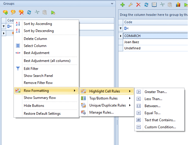
The user can determine conditional formatting for any column. To do so, it is necessary to click the right mouse button in a column header, indicate Row Format option with the cursor and select one of the following options:
- Highlight cell rules (such as, e.g., Less Than.., Between…, Equal To…)
- Data bars (allowing for marking values with different width and colors of bars)
- Color scales (coloring rows with different colors)
- Icon sets
Option Manage Rules opens a new window which displays all rules defined on the list. The window allows for adding new rules and editing or deleting of already existing rules. Here it is also possible to determine the order of executing rules on a given list.
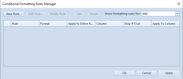
A new formatting rule can be added with the use of [New Rule] button.
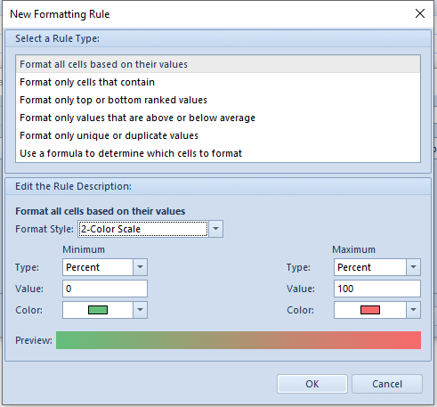
A new formatting rule window contains the following options:
- Available rule type options:
- Format all cells based on their values – all cells from a formatted column will be equated to scale specified in the rule. Only for this formatting type it is possible to determine comparative scale. This formatting does not allow for applying rule to entire row
- Format only cells that contain – only cells satisfying the rule condition are formatted. This formatting allows for applying formatting style to entire row
- Format only top or bottom ranked values – this option formats first or last values of cells from a given column. This option allows specifying how many cells should be formatted. It is possible to apply formatting to entire row
- Format only values that are above or below average – average from values of cells of a given column is calculated and values above and below that average are formatted, respectively. This option allows for formatting entire row
- Format only unique or duplicate values – this option formats only those cells which have unique or duplicate values within entire column
- Use a formula to determine which cells to format – this option allows for creating own complex algorithm for formatting cells. It is possible to apply formatting to entire rows
- Available rule description options:
- On the basis of scale – option available only for type Format all cells based on their values. It allows for selecting 2-color scale, 3-color scale, data bar or icon set for graphic presentation of data. The most important possibility is specifying a scale in percentage or numeric formats in any ranges. The formatting applies only to cells from a given column – it cannot be applied to entire rows
- On the basis of cell values – option available for all the other formattings. It is used to specify font, its color, font style settings (bold, italics, underline, etc.) and cell background. Predefined formats are also available. It is possible to apply formatting to entire rows
In the upper right corner of the rule manager window, there is a selection field enabling filtering of rules for each column from the list separately.
- For quantity equal to 0, row text will be displayed in bold and in red – must be applied to entire row
In Quantity column header, open context menu with the use of right mouse button and select option Row Formatting. From the displayed menu, choose Highlight Cell Rules and then Equal To….
In the first field of the opened window, specify value to which all values from rows of column Quantity will be compared.
For the formatting to be applied to entire row, option Apply formatting to an entire row must be selected.
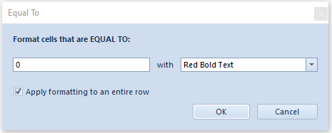
Formatting style can be selected form the list of predefined styles. Select style Red Bold Text. Click [OK] for the changes to be applied.
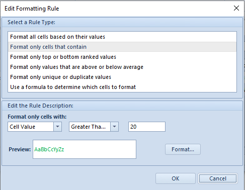
- For quantity greater or equal to 20, row will be displayed in green – must be applied to entire row
In Quantity column header, open context menu with the use of right mouse button and select option Row Formatting. From the displayed menu, choose Manage Rules.
In order to add a new rule, select [New Rule] and then the option Format only cells that contain. In the bottom part of the window in drop-down lists, set Cell Value and Greater Than or Equal To. In the displayed field, enter value to which values from rows will be compared – in this particular case, 20.
Next, open the window for selecting cell formatting by clicking on the button [Format]. According to the mentioned requirement, set font color to green.
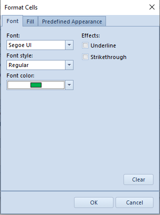
Confirm addition of the new rule by selecting [OK].
In the window for managing rules, it is also necessary to select option Apply to the row so the formatting pertains to entire row.
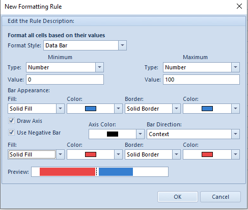
- For available quantity, add data bar presenting in graphic form available resource on a scale from 0 to 100
Upon opening context menu of Quantity column and selecting Row Formatting, choose option Data Bars. Select one of the available bars. In the new window, specify the scale. Set type Number for Minimum and Maximum and scale from 0 (Minimum) to 100 (Maximum). Set any colors for the data bar.
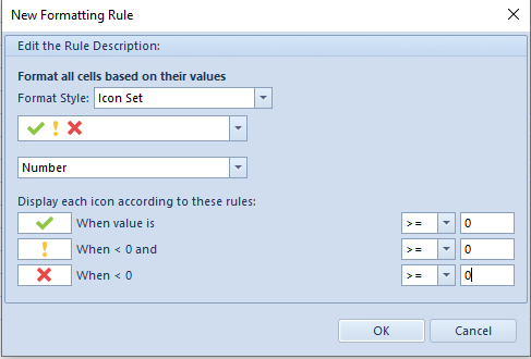
- Items with 0.00 subtotal price should be marked with red X sign
Open context menu for column Subtotal and select Row Formatting. For option Icon Sets choose ![]() from group Symbols and set type Number.
from group Symbols and set type Number.
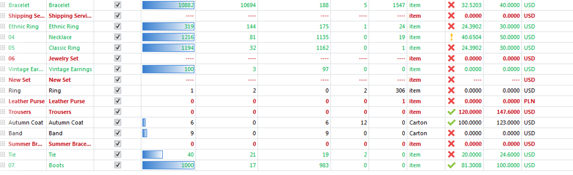
After all the defined rules are applied, the list of items should look as follows: